Select on RRR bitvector
Currently, I am working with Rayan Chikhi and two students on a library for bioinformatics that uses a bitvector to store information and rank and select operations to interrogate it. As our bitvector can be composed of $4^{64}$ bits, we have to represent in a compacted or compressed way. During my readings on bitvectors I found the papers of Raman, Raman and Rao (that’s why RRR) in SIM-SIAM symposium in 2002 and ACM Transactions on Algorithms in 2007. This is not the bitvector that we are currently using but the technics for performing rank and select in constant time are very interesting.
The details of the datastructure are very hard to understand but thankfully to Alex Bowe, the rank operation datastructure have been explained in a previous blogpost. However, as far as I know, there is no vulgarization articles on the RRR select datastructure. I think that is because of the difficulty to understand the original papers, the fact that the datastructure do not looks like “a practical solution” and because there are some fast implementations that use less space (Implementation from Navarro here or SDSL logarithmic implementation (line 448 to 534)).
So, in this post, I will only focus on the select datastructure and the representation of the bitvector as it is needed for the select query.
Rank and Select
First let’s describe the rank and select operations on a bitvector $b$ of size $m$ where $b_i$ is the $i^{th}$ bit of the vector. The operations are described as follow:
- $rank_{1}(i) = \sum_{j=0}^{i}{b_j}$ : Count the number of 1 from the beginning of the vector to the ith position.
- $rank_{0}(i) = i - rank_{1}(i)$ : Count the number of 0 from the beginning of the vector to the ith position.
- $select_{b}(i) = min(x | rank_{b}(x) == i)$ : Return the position of the ith bit set to $b$.
For this post, I will assume that there is a majority of 0 in the bitvector and that we want to perform rank and select operations on bits set to 1. Of course, everything is symmetrical, so it’s easy to replace the 1s by 0s.
Bitvector structure
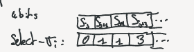
A bitvector has two main parameters: its size and the number of bit set to 1. I will call $m$ the size of the bitvector and $n$ the number of 1. By definition, a fully explicit bitvector occupy $m$ bits into memory. The RRR bitvector is sliced into small blocks of equal size $u$ (For optimality in the article $u = { {1}\over{2} } lg\,m$). Each block represent a chunk of the bitvector that we call $b_i$ and there are $p$ blocks ($p = m / u$). For a block $b_i$, we call $i$ the block number.
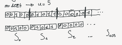
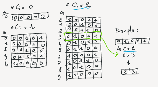
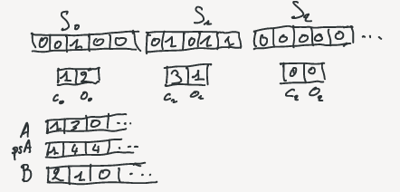
Each of the $S_i$ can be represented by two integers: the number of bit set to 1 $c_i$ and an offset identifier ($o_i$). The number of bit set is also called class of the chunk. The are exactly ${u\choose c_i}$ different possible blocks containing $c_i$ bit set to 1. Imagine that all these possible blocks are sorted lexicographically, then $o_i$ is the position of the block in that order.
For each block, storing $c_i$ take exactly $\lceil lg\,u \rceil$ bits regardless the block. Storing $o_i$ take $\lceil lg{b\choose c_i} \rceil$ bits. So, the amount of bit needed for a block depends on its class. The values for all $c_i$ and all $o_i$ are computed in two respective arrays $A$ and $B$. A prefix sum array is also computed on A where $ps_A[i] = \sum_{j=0}^{i-1}{A[j]}$. $A[i]$ corresponds to the number of 1s in the $i^{th}$ block, so $ps_A[j]$ stores the number of 1s from the beginning of the vector up to the block j-1. So, $ps_A[j]$ stores the rank of the last bit of the block j-1. It means that $ps_A[i] = rank(i \times u)$. $ps_A$ will be used as constant time access to rank values for blocks.
Construction of the select datastructures
For rapid select operations some of the values are precomputed and used as anchors for the search. Instead of having select precomputed on regular indexes all along the vector, the RRR datastructure compute regular select values:
- $C[0] = 0$
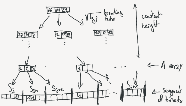
- $C[i] = \lfloor {select(i \times c) \over u} \rfloor$, with $c = (lg\,p)^2$ (defined by the authors)
By regular select values I don’t mean “the same number of bits” between two consecutive precomputed values but “the same number of 1s” (exactly $c$ 1). Dividing the select value by u, the size of a block, keeps track of the block numbers instead of the bit positions themselves.
We are now using the values of $C$ to consider the whole vector as a succession of segments from $\sigma_0$ to $\sigma_x$, where $\sigma_i$ is the segment that starts at the block $C[i]$ and ends at block $C[i+1]-1$. The segments can vary in size and we split them into two categories “sparse” and “dense”. $\sigma_i$ is called sparse if it contains at least $(lg\,p)^4$ bits (either 0 and 1), dense otherwise. In sparse segments, the block numbers of the selects are explicitly stored. To save space, the numbers are stored relatively to the beginning of the segment.
For dense segments, a tree datastructure is created with a branching factor of $\sqrt{lg\,p}$. So, because by definition of the dense segment, there are at most $(lg\,p)^4$ bits, the height of the tree is bounded by a constant. The tree structure is defined as follow:
- A leaf per block of the segment that points to the segment.
- Non leaf nodes store arrays of the size of the branching factor. Each cell contains the numbers of bit set to 1 in the corresponding subtrees.
(Almost ?) O(1) select requests
Let’s consider that we want to perform a request select(x), where $0 <= x <= m$. The global idea is that the select value will be computed in 3 main steps before joining them together:
- search for the rigth segment
- search inside of the segment for the right block
- search inside of the right block for the rigth bit.
- sum the bit position, the block position and the segment position for the global position of the select. All these points are detailed in the followind figure/description pair.
-
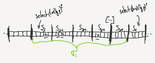
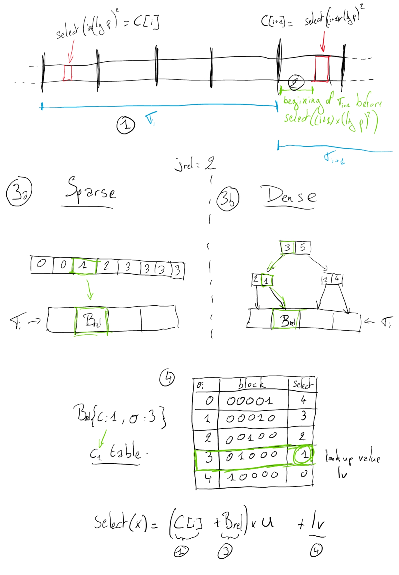
First, find the block segment where the select belongs to. To do so, compute $i= \lfloor x / \lfloor (lg\,p)^2 \rfloor \rfloor$. Because of the regular select values precomputed, we know that the select value should be part of $\sigma_i$ or the beginning of the first block of $\sigma_{i+1}$.
-
Look at the first block of $\sigma_{i+1}$ before the index of $select((i+1)(lg\,p)^2)$ (The green section on the above schema). If $rank(C[i+1] \times u) > (i+1) \times (lg\,p)^2$ (ie. $ps_A[C[i+1]] > (i+1) \times (lg\,p)^2$), the value is contained in $C[i+1]$
- If the value is part of $\sigma_i$:
- If $\sigma_i$ is sparse, go to the beginning of the sparse segment datastructure. The relative indexes of the blocks containing the ones are explicitly stored. So, first get the relative select value by doing $r = x - ps_A[i]$. Then get the relative block number of the block of interest with $j_{rel} = \sigma_i[r]$. Finally the absolute index of the bloc is obtained by doing $j_{abs} = C[i] + j_{rel}$. The selected bit is inside of the block numbered $j_{abs}$.
- If it’s dense, go to the root of the tree for $\sigma_i$.
As for the sparse block, we are looking for a relative number $j_{rel}$ from the beginning of the segment.
If the current node of the tree is $n$, $n[x]$ is the $x^{th}$ cell of the array in the node.
Search for the cell $i$ such as $n[i] \leq j_{rel} < n[i+1]$.
This search is easily done in log time as the nodes are partial sum arrays.
The following note discuss about a constant time search.
Go to the corresponding subnode and recursively do the search until you reach a leaf.
The leaf is $j_{rel}$.
Similarly to sparse blocks, $j_{abs} = C[i] + j_{rel}$.
Note: As I just described, the search into a node partial sum array is performed in log time. This leads to a non constant query time. In the RRR article the authors claim “This can be done in constant time using a lookup table”. They also say that the whole structure can be stored in $O(\sqrt{lg\,p}\,lg\,lg\,p)$ but without further explanations. In my mind, the only way to do it in constant time is to explicitly create one cell per possible select value at each level of the tree. Because a segment is created with $(lg\,p)^2$ bit set to 1, the arrays are of size $(lg\,p)^2$. This is not the same amount of memory than in the paper. So, if you, the reader, are able to explain how to constant time query in this space, please contact me !
- We now know the block $b_{j}$ from the step 3. Inside of the block we have to extract the relative bit position $k$. Here, everything is precomputed in a huge lookup table. With the class and the offset of the block, we can directly jump to the precomputed row and then to the column corresponding to the selected bit inside of the block.
Finally, the select value is the sum of position of the position of the selected segment, the relative index of the block inside of the segment and the relative position of the bit inside of the block:
$select(x) = (C[i] + j_{rel}) \times u + k$
Remarks
This blogpost is only due to my curiosity on bitvector datastructure theory. But I think that this structure is not practical. Many improvements have be done since the first publication of this work. The purpose of the blogpost is only the clarification of the technics as the scientific papers about RRR are very complicated to read and no one seems to have already published vulgarization articles on RRR select.
To understand and write this post, I was helped by Rayan Chikhi. I thank him a lot for his time and the great help. I thank also Pierre Marijon, Antoine Limasset and Camille Marchet for their proofreading.
Comments
No comments found for this article.
Join the discussion for this article on this ticket. Comments appear on this page insteantly.